
ANSYS Fluent's Solidification & Melting model makes PCM simulation accessible, but accessible doesn't mean straightforward. Accurate results depend on correct material property inputs, appropriate mesh density, proper solver configuration, and a well-calibrated mushy zone constant. Get any one of those wrong and you'll either see divergence or results that look plausible but are physically wrong.
This guide walks through the full setup process, covering what to prepare, how to configure the model, which parameters matter most, and how to troubleshoot the most common failure modes.
Key Takeaways
- ANSYS Fluent models PCM phase change using the enthalpy-porosity method, which assigns a liquid fraction (0 to 1) to each cell rather than tracking a sharp melt boundary
- Three material inputs are required: solidus temperature, liquidus temperature, and Pure Solvent Melting Heat (latent heat)
- The mushy zone constant (A_mush) is the most commonly misconfigured parameter. Validated ranges span 10⁴ to 10⁸ depending on PCM and geometry
- Always run a mesh independence study and time step sensitivity check before interpreting results
- PCM simulations are inherently transient; a steady-state solver produces meaningless output
What You Need Before Running a PCM Simulation
Before touching Fluent, confirm you have the following in hand.
Validated Thermophysical Property Data
Using generic or estimated property values is the leading cause of inaccurate results. At minimum, you need:
- Solidus and liquidus temperatures (from material datasheet or peer-reviewed source)
- Latent heat of fusion (in J/kg)
- Density — separate values for solid and liquid phases
- Thermal conductivity — solid and liquid (note: n-octadecane has 0.3 W/m·K solid vs. 0.15 W/m·K liquid — a 2:1 difference that matters)
- Dynamic viscosity of the liquid phase
- Thermal expansion coefficient (β) for Boussinesq natural convection modeling
For common PCMs: Rubitherm RT42 and RT28HC have official datasheets. For n-octadecane, the 2019 thermophysical property review by Faden et al. is a strong reference with validated property correlations.
Software and Computational Requirements
- The Solidification & Melting model is available in Fluent 16 and later
- Ensure sufficient RAM and CPU cores — transient PCM simulations are computationally heavier than steady-state cases because each time step must iterate to convergence
- Enable autosave checkpointing; full melt/solidification cycles can require thousands of time steps, and mid-run recovery saves significant time if a job fails
Geometry and Physics Readiness
Once your properties and solver setup are confirmed, lock in your domain geometry before building — changes here after meshing are costly. Decide on dimensionality based on your physics:
- 2D is acceptable when geometry and boundary conditions are symmetric and flow is laminar
- 3D is required for complex enclosure shapes or when out-of-plane convection effects are significant
How to Simulate PCM Solidification & Melting in ANSYS Fluent
Step 1: Geometry and Mesh Setup
Define the simulation domain to match the physical PCM enclosure. Typical enclosures are rectangular cavities, cylindrical containers, or square cells.
Mesh strategy:
- Refine cells near heated walls and the expected melt front region
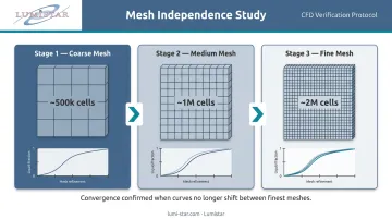
- A 2024 study in the International Journal of Thermofluids used meshes ranging from 500,000 to 2,000,000 cells and verified mesh independence by comparing liquid fraction curves over time — not just residuals
- A separate 2024 enthalpy-porosity study compared liquid fraction profiles across 2.2k, 6.6k, and 11.8k elements in 2D before scaling to 3D meshes over 2 million elements
Run a mesh independence study. Compare melting fraction curves across at least three mesh densities. If the curves converge (i.e., don't shift meaningfully between the two finest meshes), your resolution is adequate.
Step 2: Enable the Solidification & Melting Model
In Fluent's Models panel, activate the Solidification & Melting model.
What this enables:
- The enthalpy-porosity formulation — each cell receives a liquid fraction (β) between 0 (fully solid) and 1 (fully liquid)
- A momentum sink term proportional to
((1 - β)² / (β³ + ε)) × A_mush × (v - v_p)that suppresses fluid velocity in solid and mushy regions - The mushy zone is treated as a pseudo-porous medium; porosity equals the local liquid fraction
Two solver settings are required before running:
- Set solver to Pressure-Based — the solidification/melting model is incompatible with the density-based solver
- Set to Transient — the melt front evolves with time; phase change has no steady-state solution
Step 3: Define PCM Material Properties
In the Materials panel, input all thermophysical properties for both solid and liquid phases.
Three phase-change-specific inputs (high priority):
| Field in Fluent | What It Represents | Example: n-octadecane |
|---|---|---|
| Solidus Temperature | Temperature at which solidification begins | ~300.8 K |
| Liquidus Temperature | Temperature at which melting completes | ~301.5 K |
| Pure Solvent Melting Heat | Latent heat of fusion (J/kg) | ~236,980 J/kg |
These values must come from validated datasheets or peer-reviewed literature for your specific PCM. Do not estimate them.
Beyond the material property table, the mushy zone constant (A_mush) is configured separately and warrants careful attention.
Mushy zone constant (A_mush):
- Controls how aggressively the momentum sink damps flow in partially melted cells
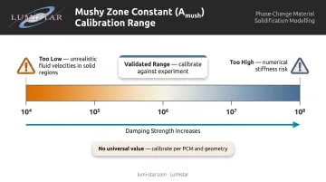
- ANSYS Fluent documentation recommends 10⁴ to 10⁷ for most computations
- Published studies have tested values up to 10⁸: Martinez et al. (Journal of Energy Storage, 2023) found 10⁴ produced realistic fusion contours but over-predicted melting speed, while 10⁵ to 10⁶ introduced numerical artifacts at the solid PCM base
- Treat A_mush as a calibration parameter, not a default
Validate your chosen A_mush value against experimental melting fraction curves for your specific PCM and geometry before finalizing it.
Step 4: Boundary Conditions and Solver Settings
Apply a constant temperature or heat flux to heated wall(s), and set remaining walls as adiabatic if insulation is assumed. Boundary condition accuracy directly governs both temperature distribution and melting rate predictions.
Solver settings — based on published validated studies:
| Setting | Recommended Approach |
|---|---|
| Pressure-velocity coupling | SIMPLE |
| Pressure discretization | PRESTO! (common in PCM literature) |
| Momentum/energy discretization | QUICK or bounded second-order |
| Transient formulation | Bounded second-order implicit |
| Energy residual | 10⁻¹² (Alam et al., Purdue 2021) or 10⁻⁵ minimum |
| Continuity/momentum residual | 10⁻⁵ |
| Under-relaxation: pressure/momentum/energy | 0.3 / 0.7 / 1.0 (Alam et al.) |
Time step selection:
- Published Fluent PCM studies have used time steps of 0.03 s (Martinez et al.) and 0.1 s (Alam et al.)
- An oversized time step lets the phase front advance unrealistically across multiple cells in one iteration; an undersized step increases computation time with little accuracy gain
- Run a time step sensitivity check — compare melting fraction curves at two different time steps before committing to a final value
Key Parameters That Affect PCM Simulation Accuracy
Simulation outcomes are highly sensitive to a small set of interacting parameters. Changing one without considering the others can produce results that look convergent but are physically wrong.
Mushy Zone Constant (A_mush)
This is the parameter most frequently misconfigured in Fluent PCM setups.
- Too low: The damping term is weak, allowing unrealistic fluid velocities in nearly solid regions
- Too high: Velocity transitions to zero too abruptly, which can introduce numerical stiffness
- A_mush is geometry- and viscosity-dependent — there is no universal correct value
- Calibrate against experimental data or published benchmarks matching your PCM and geometry
Latent Heat of Fusion and Phase Change Temperature Range
The latent heat value (entered as Pure Solvent Melting Heat) determines how much energy is absorbed per kilogram during melting. An incorrect value shifts the entire melting timeline.
A very narrow solidus-to-liquidus temperature range — common in pure substances — creates numerical stiffness. If you observe oscillations in the liquid fraction field, widening the phase change range slightly (if physically justifiable) can improve stability.
Mesh Resolution in the Phase Change Zone
The enthalpy-porosity method distributes phase change across cells in the mushy zone. Under-resolved meshes create two specific problems:
- Oversized cells: The mushy zone appears artificially thick, misrepresenting heat transfer rates and melting time predictions
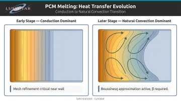
- Coarse near-wall resolution: Early-stage conduction-dominated heat transfer is poorly captured where thermal gradients are steepest
Refine the mesh near heated walls before running production simulations, especially if your PCM has a narrow phase change range.
Natural Convection: Boussinesq Approximation
As melting progresses, buoyancy-driven flow takes over from conduction as the dominant heat transfer mechanism in the liquid PCM. This is modeled using the Boussinesq approximation, which requires the thermal expansion coefficient (β) of the liquid phase.
- Alam et al. used β = 0.001 K⁻¹ for RT35 in a validated Fluent study
- For liquid n-octadecane, a 2024 thermophysical property study reports β ranging from 9.03×10⁻⁴ to 9.55×10⁻⁴ °C⁻¹ between 30°C and 90°C
If β is unavailable for your specific PCM, use differential scanning calorimetry (DSC) data or cross-reference against a chemically similar substance from validated literature.
Common Mistakes and Troubleshooting
Running the Solver in Steady-State Mode
PCM melting and solidification are time-dependent processes. Steady-state mode cannot represent the evolving liquid fraction field and will produce results with no physical meaning. Always use Transient solver mode.
Skipping Mesh and Time Step Sensitivity Studies
Many users accept first-run results without checking whether mesh density or time step size is influencing the output. Before reporting any melting fraction curves:
- Compare results across at least two mesh densities
- Compare results across at least two time step sizes
- Results should be stable before being treated as valid
Those same mesh and time step choices are often the first place to look when a simulation starts misbehaving.
Divergence or Oscillating Residuals
If residuals diverge or oscillate, check these in order:
- A_mush too low — increase by one order of magnitude and re-run
- Oversized time steps — reduce the step size and check whether convergence improves
- Under-relaxation factors too aggressive — tighten pressure (try 0.3) and momentum (try 0.7)
- Energy residual target too loose — tighten to at least 10⁻⁵; established PCM studies often target 10⁻¹²
Liquid Fraction Not Reaching 1.0
If the simulation ends before full melting despite adequate heat input, check:
- Simulation end time set too short — extend it
- Boundary condition not sustained throughout the simulation
- Latent heat value entered too high — verify against the material datasheet
- Heat flux or temperature boundary condition lower than the liquidus temperature
Working through these checks in order — from solver mode and mesh setup to convergence and boundary conditions — covers the vast majority of issues encountered in PCM simulations.
Conclusion
The enthalpy-porosity method has been the standard for PCM phase-change simulation since Voller and Prakash's 1987 fixed-grid formulation — the model itself isn't the weak point. What separates credible simulations from misleading ones is the workflow around it: validated material inputs, appropriate mesh resolution, calibrated A_mush, and sensitivity checks on both mesh and time step.
The most common simulation failures don't come from the model. They come from skipped validation steps. Comparing simulated liquid fraction curves against published experimental data — and reporting the deviation quantitatively — turns a Fluent PCM simulation into a result an engineer can actually stand behind.
Frequently Asked Questions
What is PCM used for?
PCMs are used wherever large amounts of heat need to be stored or released at near-constant temperature. Applications include building thermal insulation, HVAC load shifting, electronics cooling, solar thermal energy storage, and aerospace thermal control.
What are the three types of PCM?
The three main classifications are:
- Organic PCMs (paraffins and fatty acids): chemically stable and non-corrosive
- Inorganic PCMs (salt hydrates): higher energy density, typically 100–300 kJ/kg, but potentially corrosive
- Eutectic PCMs: mixtures engineered to melt at a specific target temperature
What are the 3 C's of heat transfer?
The three heat transfer mechanisms are conduction (heat flow through solids via molecular interaction), convection (heat transfer via fluid motion, which dominates in liquid PCM after initial melting), and radiation (electromagnetic energy transfer, typically secondary in PCM enclosure simulations but not negligible at high temperatures).
What is the enthalpy-porosity method in ANSYS Fluent?
It's Fluent's numerical approach for modeling PCM phase change. Rather than tracking a sharp melt boundary, it assigns a liquid fraction (0 to 1) to each cell based on an enthalpy balance and treats the partially melted mushy zone as a porous medium. The melt interface is not tracked explicitly: it emerges from the liquid fraction field.
What is the mushy zone constant and how do I choose it?
A_mush controls the strength of the momentum damping applied to partially melted cells. Fluent recommends values between 10⁴ and 10⁷ for most cases, but published studies test up to 10⁸. The correct value is PCM- and geometry-specific — calibrate it by comparing your simulated melting fraction curves against experimental or benchmark data.
How do I validate my PCM simulation results in ANSYS Fluent?
Compare simulated liquid fraction vs. time curves and temperature contours against published experimental data for the same PCM and geometry. Alam et al. reported local temperature agreement within 2 K of experiment; Hosseinpour et al. reported an average difference of 2.4% against validation data. Use those as benchmarks for what "good" agreement looks like.