Introduction
LDPC decoder design demands expertise across error-correction theory, digital hardware architecture, and implementation trade-offs — algorithm selection, parallelism strategies, and platform-specific constraints all have to align before a single bit moves through the system correctly.
FPGA/ASIC designers, DSP hardware engineers, and systems engineers working across 5G, Wi-Fi, aeronautical telemetry, and flight test instrumentation all encounter the same hard truth: a poorly designed LDPC decoder doesn't just underperform. It produces error floors, fails throughput targets, or overruns silicon area budgets — problems that require costly re-spins to fix.
This guide walks through the full design and implementation process, from algorithm selection and prerequisite decisions through RTL design, verification, and the three failure modes that derail first-time implementations.
Key Takeaways
- Algorithm choice (Sum-Product vs. Min-Sum) directly sets hardware complexity; Min-Sum wins on real hardware for its implementation simplicity
- Quasi-cyclic (QC) parity-check matrix structure determines parallelism, memory layout, and barrel-shifter requirements
- Check Node Units (CNU) and Variable Node Units (VNU) are the core building blocks; all other logic supports their operation
- Layered decoding cuts required iterations by about half versus flooding, but requires careful management of layer-to-layer data dependencies
- Verification must cover both BER waterfall behavior and timing closure; missing either leads to silent system failures
LDPC Decoder Architecture: Core Concepts and Design Scope
An LDPC decoder takes a noisy received codeword and recovers the original transmitted bits. It does this by iteratively exchanging soft-decision messages between two sets of nodes in a bipartite graph — the Tanner graph — whose structure is defined by the sparse parity-check matrix H.
The Two Fundamental Processing Units
Every LDPC decoder architecture is built around two units:
- Check Node Unit (CNU): Enforces parity constraints by computing check-to-variable messages; aggregates incoming variable-to-check messages and outputs updated reliability estimates per connected variable node.
- Variable Node Unit (VNU): Aggregates incoming check-to-variable messages along with the channel log-likelihood ratio (LLR) and outputs updated variable-to-check messages.
All architectural decisions — memory layout, interconnect topology, pipeline depth — flow from how these two units are constructed and connected.
That construction directly determines which scheduling approach is viable — and scheduling is where architectures diverge most.
Architectural Families
Three main scheduling approaches exist, and choosing between them affects everything downstream:
| Architecture | Message Update Order | Iterations to Converge | Hardware Complexity |
|---|---|---|---|
| Flooding | All nodes simultaneously | Baseline | Moderate |
| Row-Layered | Row by row (check nodes) | ~Half of flooding | Higher |
| Column-Layered | Column by column (variable nodes) | ~Half of flooding | Higher |
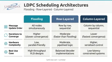
Layered decoders converge in roughly half the iterations of flooding for the same BER target — which translates directly to higher throughput at the same clock rate, making them the default choice for performance-constrained implementations.
Design Prerequisites: Algorithm, Code Structure, and Platform
Before writing a single line of RTL, four decisions must be locked down. Getting any of them wrong forces architectural rework.
Specify the Target Code Completely
The LDPC code parameters dictate everything:
- Block length (N) and code rate (K/N)
- Parity-check matrix structure: random vs. quasi-cyclic (QC)
- Standard compliance: DVB-S2 uses normal FECFRAMEs of 64,800 bits; 5G NR base graph 1 supports code blocks up to 8,448 bits; IRIG 106 defines QC-LDPC codes at rates 1/2, 2/3, and 4/5 with block sizes of 1,024 and 4,096 bits
These parameters set memory requirements, CNU/VNU fan-in, and the parallelism ceiling.
Choose the Decoding Algorithm
Two algorithms dominate:
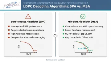
- Sum-Product Algorithm (SPA): Near-optimal BER performance. Requires log-domain or LUT-based computation of hyperbolic tangent functions in the CNU — expensive in hardware.
- Min-Sum Algorithm (MSA): Replaces those nonlinear operations with simple comparisons and sign-bit XOR. Scaled and offset variants (Normalized MSA, Offset MSA) close most of the BER gap at minimal additional logic cost.
MSA variants dominate hardware implementations. Offset MSA typically recovers 0.2–0.4 dB of the BER gap versus SPA at the cost of a single subtraction per message, making it the pragmatic default for most designs.
Hardware Platform Readiness
- FPGA: Reconfigurable, faster time-to-silicon, but limited DSP and BRAM resources constrain parallelism. One verified FPGA implementation of an 802.11n QC-LDPC decoder achieved 608 Mb/s at 260 MHz.
- ASIC: Custom memory macros and logic libraries eliminate FPGA routing overhead. A 65 nm CMOS implementation of the same 802.11n code achieved 15.8 pJ/bit/iteration energy efficiency, a figure out of reach for FPGA fabric.
Fix the LLR Quantization
Fixed-point bit-width for LLR messages trades BER performance against memory and arithmetic area. A DVB-S2 finite-precision study found that 6-bit quantization produces approximately 0.1 dB performance degradation versus higher-precision decoding. Four to six bits covers the practical range for most implementations.
Standards Compliance Locks Parameters Early
For programs operating within a defined standard — particularly aeronautical telemetry systems that must comply with IRIG 106 — the code parameters are fixed by the standard, not freely chosen.
Lumistar's LS-28-DRSM series and LS-18 series receivers implement LDPC decoding across all six IRIG 106 codes — rates 1/2, 2/3, and 4/5 at both 1,024 and 4,096 bit block sizes. For flight test programs that don't need a bespoke decoder, this eliminates custom design risk entirely.
How to Design and Implement an LDPC Decoder: Step-by-Step
Decoder implementation follows a fixed sequence: algorithm definition → architecture design → RTL coding → synthesis → verification. Shortcutting any phase reliably produces costly re-spins.
Step 1: Define the Architecture and Parallelism
For QC-LDPC codes, the cyclic shift structure of the parity-check matrix directly sets the parallelism options. Each circulant sub-matrix has size Z × Z (the lifting factor), and a fully parallel architecture instantiates Z CNU/VNU pairs per layer. Increasing Z raises throughput proportionally but also multiplies logic and routing area.
Scheduling decision:
- Flooding: All check and variable nodes update simultaneously. Simple to implement, but convergence is slow.
- Layered (row or column): Processes one layer at a time, updating messages before moving to the next. Achieves equivalent BER performance in half the iterations — confirmed across multiple published implementations.
The layer-to-layer data dependency is the critical complication. Each layer reads messages written by the previous layer, so pipelining between layers introduces an approximation. Published column-layered implementations show this pipelining causes less than 0.02 dB BER degradation , an acceptable trade for the clock speed improvement.
Step 2: Design the Check Node and Variable Node Units
CNU design (Min-Sum):
The CNU must:
- Find the two minimum magnitudes among all incoming variable-to-check messages
- Compute the XOR of all incoming sign bits
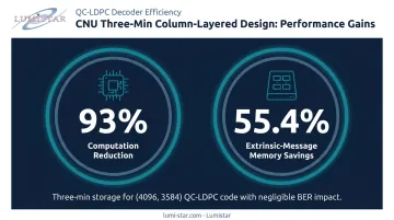
Storing only the top-2 (or top-3) sorted magnitudes per check node dramatically reduces memory versus storing all messages. A three-min column-layered implementation reports 93% computation reduction for a structured (4096, 3584) QC-LDPC code with (4,32) regularity, with 55.4% extrinsic-message memory savings from the three-min storage approach — with negligible BER impact.
VNU design:
Variable nodes sum incoming check-to-variable messages and the channel LLR. For multi-Gb/s targets, carry-save adder trees minimize critical path delay when accumulating multiple messages in parallel. At high throughput, ripple-carry implementations cannot close timing — carry-save is the practical choice.
Step 3: Design the Interconnect and Memory Architecture
Interconnect:
For QC codes, barrel shifters implement the cyclic permutations defined by H. The column-layered approach places barrel shifters before and after the VNU array to map messages between row order and column order. Barrel shifter placement determines both the critical path and routing congestion , so plan their location early in the floorplan.
Random LDPC codes require full crossbar-style interconnects. This is why QC codes are strongly preferred for hardware: the cyclic permutation structure makes routing tractable.
Memory architecture:
Three categories of storage are required:
- Channel LLR messages (intrinsic)
- Check-to-variable extrinsic messages
- Intermediate sorted magnitude vectors (for top-k min storage)
Layered decoders reuse message memory more efficiently than flooding. Hocevar's layered decoding work reports 45–50% reductions in memory bits and instances versus flooding while maintaining the same throughput and error performance.
Step 4: RTL Coding, Synthesis, and Timing Closure
Write CNU, VNU, barrel shifters, and the layer controller as separate modules in VHDL or Verilog. Set synthesis constraints (clock period, area targets, fanout limits) before running synthesis. Constraints defined post-synthesis rarely produce a clean first pass.
Timing closure is iterative. Common interventions:
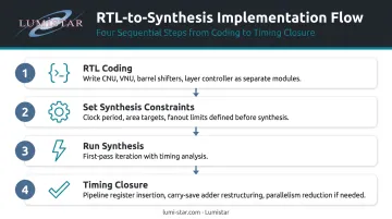
- Insert pipeline registers at CNU comparator chain boundaries
- Restructure VNU adder trees (carry-save, not ripple-carry)
- Reduce parallelism or target clock if area budget is exceeded
Plan for at least two synthesis iterations. A first-pass 500 MHz target on a 28 nm node, for example, will typically require one round of register insertion before the critical path closes cleanly.
With these four steps complete, the decoder architecture is ready for functional simulation and hardware-in-the-loop verification against known BER curves.
Post-Implementation Verification and Testing
Verification has two independent dimensions: algorithmic correctness and implementation correctness. Both must pass before deployment.
Functional and BER Verification
Compare RTL decoder output against a floating-point software reference decoder running the same received frames under the same channel conditions. BER vs. Eb/N0 curves must match the expected waterfall behavior within tolerance — typically within 0.1–0.2 dB of the reference.
A mismatch almost always points to one of three causes:
- Sign-bit handling error in the CNU
- Incorrect barrel shifter permutation index
- Quantization overflow in the VNU accumulator
Timing and Resource Verification
Post-place-and-route timing reports must confirm positive setup and hold slack at the target clock. For FPGAs, check that resource utilization stays within budget across all resource types:
- LUT, BRAM, DSP counts must not exceed device limits
- Parallelism level may need reduction if LUT budget is exceeded
- Memory organization may need restructuring if BRAM is over-allocated
Exceeding resource limits calls for architectural changes, not constraint tweaks.
Silent Failures in Deployed Hardware
A decoder can pass basic functional tests while producing BER degradation of multiple orders of magnitude at low SNR. Sign-bit bugs in the CNU produce valid-looking output at high SNR where errors are rare, then fail completely at operating SNR. Quantization overflow causes the same pattern. Both failure modes are silent in deployed hardware — undetectable until link margin runs out.
Run full BER curves on post-synthesis simulation before tapeout or deployment. This is the only step that reliably surfaces sign-bit and overflow bugs before they reach the field.
Common LDPC Decoder Design Problems and How to Fix Them
Critical Path Violation in the CNU or VNU
Synthesis fails to meet timing at the target clock frequency. The culprit is usually combinational path length: comparator chains for minimum-magnitude selection in the CNU, or multi-operand adder trees in the VNU.
To resolve it:
- Insert pipeline registers between CNU stages (between horizontal pass steps in layered decoders)
- Restructure VNU adder trees using carry-save addition
- Accept 1–2 additional pipeline cycles per layer — this rarely exceeds the latency budget
Error Floor Appearing at High SNR
The BER curve flattens or rises at low error rates instead of continuing to fall. Three root causes account for most cases: LLR quantization is too coarse, the stopping criterion exits too early, or the Tanner graph has trapping sets that iterative decoding cannot resolve.
Start with the quick fixes:
- Increase LLR quantization by 1–2 bits and re-run BER simulation
- Raise the maximum iteration count
If the floor persists, investigate whether the code has known trapping sets at the target rate. Richardson's error-floor analysis provides the systematic framework for that evaluation.
Memory Bandwidth Bottleneck Limiting Throughput
The decoder cannot sustain target throughput even when CNU/VNU utilization looks healthy. In a fully parallel architecture, simultaneous accesses often map to the same memory bank — the resulting conflicts stall the pipeline regardless of compute capacity.
Two structural fixes address this directly:
- Restructure memory into interleaved banks aligned to the QC sub-matrix access pattern
- For row-layered decoders, store each layer's messages in dedicated banks to enable conflict-free parallel access across the full layer width
Frequently Asked Questions
What is an LDPC decoder?
An LDPC decoder is a hardware or software circuit that recovers original transmitted data from a noisy received signal. It iteratively passes soft-decision reliability messages between variable nodes and check nodes — as defined by the code's sparse parity-check matrix — until a valid codeword is found or the maximum iteration count is reached.
What is the difference between an encoder and a decoder?
The encoder takes original message bits and adds redundant parity bits to produce a longer codeword for transmission. The decoder operates at the receiver — it takes the noisy received codeword and uses those redundant bits to detect and correct errors, recovering the original message.
What is the difference between Reed-Solomon and LDPC?
Reed-Solomon codes operate on multi-bit symbols using algebraic hard-decision decoding and handle burst errors well. LDPC codes operate on individual bits using iterative soft-decision belief-propagation decoding and approach the Shannon channel capacity limit. LDPC is preferred in modern systems where SNR efficiency is the priority.
What decoding algorithm is most commonly used in hardware LDPC implementations?
The Min-Sum Algorithm (MSA) and its scaled/offset variants dominate hardware implementations. They replace the computationally expensive logarithm and hyperbolic tangent operations of the Sum-Product Algorithm with simple comparisons and additions, reducing hardware complexity with minimal BER penalty.
What is the difference between row-layered and column-layered LDPC decoding?
Both partition the parity-check matrix into layers and update messages layer by layer rather than all at once. Row-layered processing updates check nodes one row-layer at a time; column-layered processing updates variable nodes one column-layer at a time. Critical path length and memory access patterns differ between the two, making each better suited to specific hardware targets.
How is LDPC decoding used in aeronautical telemetry systems?
IRIG 106 defines QC-LDPC codes for telemetry systems at rates 1/2, 2/3, and 4/5 with block sizes of 1,024 and 4,096 bits. Ground station receivers must implement compliant LDPC decoders to recover telemetry data from airborne transmitters, particularly at long range and low SNR conditions typical of flight test environments.