Introduction
When an FM signal arrives at your receiver, the original message is encoded entirely in the carrier's instantaneous frequency — not its amplitude. Recovering that message accurately is FM demodulation. As defined by the FCC under 47 CFR 73.310, the carrier's instantaneous RF frequency varies in direct proportion to the amplitude of the modulating signal. Demodulation reverses that relationship.
This matters across a wide range of systems — FM broadcast radio (88–108 MHz), aeronautical telemetry under IRIG 106, FMCW radar altimeters, and two-way radio communications all depend on it.
The concept is straightforward. Getting it right is not. Demodulation quality varies significantly based on which technique you choose, how well you know your carrier and deviation parameters, and whether each processing stage is configured correctly. This guide covers each stage: baseband mixing, demodulation technique selection, scaling, and troubleshooting.
Key Takeaways
- FM demodulation recovers the message signal by measuring how the carrier's frequency changes over time.
- Four core stages: mix to baseband → low-pass filter → extract instantaneous frequency → scale and recover the message.
- Three primary DSP techniques — polar discriminator, atan2 + FIR derivative, and PLL — each involve different trade-offs in complexity, noise tolerance, and latency.
- Critical parameters: carrier frequency accuracy, peak deviation, modulation index, sample rate, and filter design.
- Most demodulation failures trace back to incorrect baseband mixing, phase wrap-around, or miscalculated scaling constants.
When to Demodulate an FM Waveform and What You Need
FM demodulation is the correct approach when the message signal is encoded in instantaneous frequency variations of the carrier. It is not the right approach for amplitude-modulated signals, PSK/QAM digital schemes, or any signal whose carrier falls outside your receiver's tunable range — applying FM demodulation to those signals produces only noise.
Common use cases include:
- FM broadcast radio (88–108 MHz, 200 kHz channel spacing, ±75 kHz peak deviation per 47 CFR 73.201)
- Aeronautical and defense flight test telemetry (IRIG 106-compliant FM/FM subcarrier channels)
- FMCW radar altimetry — far more common than pulsed altimeters in civil aviation
- Seismic monitoring and two-way radio communications
In flight test telemetry, IRIG 106 Chapter 3 defines FM/FM proportional-bandwidth channels at ±7.5%, ±15%, and ±30% deviation, plus constant-bandwidth channels from ±2 kHz to ±256 kHz — making FM demodulation a core requirement across most range operations.
Signal and System Requirements
Before you start, confirm you have:
- Known carrier frequency and peak deviation (Δf) — both must be accurate
- Complex I/Q samples — either from direct SDR capture or analog downconversion; FM demodulation in DSP requires complex baseband input
- Adequate sample rate — higher than the Nyquist minimum to maintain phase stability and filter roll-off headroom
- A processing platform — MATLAB, GNU Radio, Python/SciPy, FPGA, or a dedicated telemetry receiver
When these requirements add up to significant integration work, dedicated receiver hardware handles them internally. Lumistar's LS-28-DRSM series, for example, performs analog downconversion and I/Q generation on-board, offers FM demodulation as a firmware-selectable personality, and covers RF bands from 200 MHz to 7 GHz — so the signal-chain stages above are already solved at the hardware level.
How to Demodulate an FM Waveform: Step-by-Step
Step 1: Mix the FM Signal to Complex Baseband
Multiply the received signal by a complex exponential exp(−j2πfct) at the carrier frequency to shift the FM signal to DC (0 Hz). When using an SDR, tune the hardware to the carrier center frequency to capture I/Q samples with the signal already near baseband.
After mixing:
- Plot the spectrum and confirm the FM signal is centered at 0 Hz
- If multiple channels are present within the capture bandwidth, apply a frequency shift to the desired channel before proceeding
- Check for I/Q imbalance artifacts (hardware imperfections can leave mirror images near baseband)
Step 2: Apply a Low-Pass Filter to Isolate the Channel
Design a low-pass filter with the passband edge set at the FM channel half-bandwidth. For commercial FM, that's 100 kHz; for telemetry channels, refer to your IRIG 106 channel specification.
FIR filters with a Hamming window are a practical default: SciPy's firwin uses Hamming by default and produces linear-phase filters that are straightforward to design and characterize.
After filtering, decimate the signal to reduce computational load for subsequent stages. Confirm no aliasing by checking the spectrum post-decimation.
Step 3: Extract Instantaneous Frequency
Two reliable approaches:
Polar discriminator method:
Compute v[n] = x[n] × x*[n−1], multiplying each sample by the complex conjugate of the previous sample. Take angle(v[n]) (atan2) to recover the phase difference, which is directly proportional to instantaneous frequency. This is how GNU Radio's Quadrature Demod block operates.
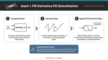
atan2 + derivative method:
- Compute phase of each I/Q sample:
atan2(Q, I) - Unwrap the phase sequence to remove ±π discontinuities
- Convolve with a derivative FIR filter
Critical: the derivative FIR introduces a group delay of (N−1)/2 samples for an N-tap filter. Apply a matching all-pass delay to any parallel processing branch before multiplication; misalignment causes phase artifacts that are difficult to diagnose.
Step 4: Recover, Scale, and Post-Process the Message Signal
Scaling is non-negotiable and method-specific:
| Method | Scaling Factor |
|---|---|
| Polar discriminator | samp_rate / (2π × deviation) |
| atan2 + FIR derivative | 1 / (2π × kf × Ts) |
After scaling:
- Apply a final low-pass filter to remove components above the message bandwidth (e.g., above 15 kHz for audio)
- Decimate again if needed to reach the target output sample rate
- Verify output by comparing the waveform shape to the known or expected message signal — a single-tone FM input should produce a clean sine wave at ±1 amplitude when normalized
FM Demodulation Techniques and When to Use Each
Pick the wrong demodulation approach and you introduce unnecessary noise, waste processing resources, or accumulate phase error that corrupts your output. Three DSP-based methods cover the vast majority of FM demodulation scenarios — here's how to choose between them.
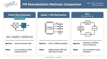
Polar Discriminator (Conjugate Multiply + atan2)
Compute the product of the current sample and the complex conjugate of the previous sample. The angle of this product equals the phase difference between consecutive samples — which is instantaneous frequency.
Formula: y[n] = arg(x[n] × conj(x[n−1]))
Normalized gain: samp_rate / (2π × deviation)
Best for: General-purpose software DSP, telemetry ground station software, and any situation where simplicity and robust noise performance matter. This method is inherently immune to ±π wrap-around for properly sampled signals and is the recommended default for most implementations.
Phase-Then-Differentiate (atan2 + FIR Derivative Filter)
Extract per-sample phase via atan2, unwrap the phase, then differentiate using a high-quality FIR derivative filter. Alternatively, compute the derivative directly from I/Q components using:
ṡ = (I·Q̇ − Q·İ) / (I² + Q²)
This avoids the atan2 computation entirely, which matters on hardware without floating-point units.
Best for: FPGA implementations where a CORDIC pipeline handles phase extraction efficiently — for example, using a vendor-supplied CORDIC IP core. Provides slightly better output SNR than the polar discriminator in high-sample-rate implementations.
Phase-Locked Loop (PLL)
A feedback loop continuously tracks the instantaneous frequency of the FM signal. The frequency correction signal from the loop filter represents the demodulated message, and loop bandwidth controls both lock range and tracking speed.
Best for: Slowly varying FM signals or situations where the carrier frequency is not precisely known ahead of time. However, PLL output amplitude is less consistent than the other methods, making it less suitable for precision telemetry measurements.
For most software-defined implementations — including telemetry ground station receivers — the polar discriminator is the practical starting point. Move to phase-then-differentiate when FPGA pipeline efficiency is a constraint, and consider a PLL only when carrier frequency uncertainty demands adaptive tracking.
Key Parameters That Affect FM Demodulation Proven Performance
Carrier Frequency and Frequency Deviation
The carrier frequency must be accurate for correct baseband mixing. Peak deviation (Δf) defines how far the instantaneous frequency swings and determines required filter bandwidth.
- US commercial FM: ±75 kHz peak deviation, confirmed by ITU-R BS.450-4 and FCC rules
- IRIG 106 telemetry: ±2 kHz to ±256 kHz for constant-bandwidth channels; ±7.5%/±15%/±30% for proportional-bandwidth channels
Impact of errors:
- Carrier frequency offset → residual sinusoidal component in demodulated output
- Underestimated deviation → output clipping or amplitude compression
- Overestimated deviation → reduced effective output SNR
Modulation Index (β)
β = Δf / fm (peak deviation divided by message bandwidth). This determines the signal's bandwidth and noise behavior.
- Narrowband FM (β << 1): bandwidth ≈ 2 × message frequency — used in two-way radio
- Wideband FM (β >> 1): uses more bandwidth but delivers far better noise immunity — standard in broadcast FM and flight test telemetry
A mismatch between assumed and actual β leads to either message bandwidth truncation or insufficient adjacent-channel rejection.
Sample Rate and Filter Design
The sample rate at the demodulation stage should be at least 5–10× the channel bandwidth. Higher sample rates provide extra margin for filter roll-off and keep phase differences between consecutive samples well below ±π.
Two filters govern performance at this stage:
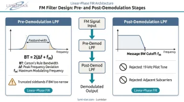
- Pre-demodulation LPF: Pass the entire FM channel bandwidth while rejecting adjacent channels. Use Carson's rule — BT = 2(Δf + fm) — to set the passband width. A filter set too narrow truncates FM sidebands and distorts the message.
- Post-demodulation LPF: Pass message bandwidth while rejecting out-of-band components (pilot tone, adjacent subcarriers). FIR filters are preferred throughout for their linear phase response.
Common Mistakes and Troubleshooting
These are the most common issues encountered during FM demodulation, along with their causes and fixes.
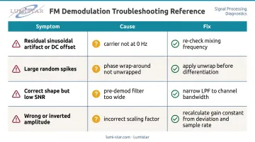
Symptom: Residual Sinusoidal Artifact or DC Offset
Cause: Signal was not correctly mixed to 0 Hz — a frequency offset remains between carrier and local oscillator.
Fix: Plot the spectrum immediately after mixing. Confirm the signal peak sits at 0 Hz. Adjust mixing frequency or retune the SDR. Also check for I/Q imbalance — hardware imperfections (amplitude imbalance, phase imbalance, DC offset) leave mirror images near baseband that look like mixing errors.
Symptom: Large Random Spikes in the Demodulated Waveform
Cause: In the atan2 method, phase wrap-around was not handled — MathWorks documents that jumps between consecutive phase angles ≥ π radians require correction by adding multiples of ±2π. Without unwrapping, these jumps become large impulses after differentiation.
Fix: Apply phase unwrapping after atan2 extraction, before differentiation. For the polar discriminator, verify the sample rate is high enough that phase differences between consecutive samples stay well below ±π.
Symptom: Correct Shape but Low SNR
Cause: Pre-demodulation filter is too wide (passing noise from adjacent channels), or an inferior demodulation technique (slope detection, zero-crossing) is in use.
Fix: Narrow the pre-demodulation LPF to match the actual channel bandwidth. Switch to the polar discriminator or atan2 + FIR method — both deliver noticeably higher SNR than FM-to-AM conversion techniques.
Symptom: Output Amplitude Is Wrong or Inverted
Cause: Scaling factor was omitted or calculated incorrectly. Each method requires a different gain constant.
Fix: Compute the correct scaling factor from the known deviation and sample rate (see Step 4 table above). Verify by feeding a single-tone FM signal and confirming the demodulated output produces a sine wave at ±1 normalized amplitude.
Frequently Asked Questions
What is frequency modulation and demodulation theory?
FM encodes a message by varying the carrier's instantaneous frequency in proportion to the message amplitude. The carrier frequency itself stays constant; only its moment-to-moment deviation changes. Demodulation reverses this by measuring how that frequency changes over time, typically through phase differentiation or phase comparison between consecutive samples.
What are the different demodulation techniques of FM?
The main DSP techniques are: polar discriminator (conjugate multiply + atan2), phase-then-differentiate (atan2 + FIR derivative), and Phase-Locked Loop (PLL). Analog methods include slope detection, delay line discriminator, and zero-crossing discriminator. The polar discriminator and atan2 + FIR methods offer the best noise performance in software implementations.
What are the real-life applications of frequency modulation?
FM is used across a wide range of applications:
- Broadcast radio and two-way radio
- Aeronautical flight test telemetry (IRIG 106)
- Seismic monitoring (USGS FM subcarrier telemetry systems)
- Assistive listening technology and magnetic tape recording
- FM sound synthesis
FM's constant-envelope property and noise immunity make it especially suitable for safety-critical and high-fidelity applications.
What is the difference between narrowband and wideband FM demodulation?
Narrowband FM (β < roughly 0.3) has a bandwidth approximately equal to twice the message frequency. It is used in two-way radio to conserve spectrum. Wideband FM (β >> 1) trades bandwidth for dramatically better SNR, which is why broadcast FM and flight test telemetry use it. The demodulation circuitry is the same for both; filter bandwidths and deviation parameters must be set to match.
What is Carson's rule and why does it matter for FM demodulation?
Carson's rule — BT = 2(Δf + fm) — estimates the effective bandwidth of an FM signal. It is used to set the width of the pre-demodulation bandpass filter. Setting the filter too narrow relative to this bandwidth truncates FM sidebands and distorts the recovered message signal.
What are the applications of modulation and demodulation?
Modulation converts a message signal for efficient transmission over a channel (radio, cable, optical fiber); demodulation recovers it at the receiver. Together they underpin FM radio, digital communications, telemetry data links, radar ranging, seismic data transmission, and any system requiring reliable signal delivery over distance.